1. Basic Tutorial

To run any model in BATMODS-lite, you will need to construct a Simulation and Experiment. All Simulation classes are constructed using a .yaml file that contains a description of the parameters. The easiest way to find out how to build a .yaml input for a given model is to get a template from bmlite.templates. When calling the templates function, pass the name of the model subpackage (case insensitive) to get a list of available templates.

import numpy as np
import bmlite as bm

bm.templates('spm')

==============================
spm templates:
==============================
  - [0] graphite_nmc532
  - [1] graphiteSiOx_nmc811
  - [2] graphite_lfp

To print a specific template, pass a second input as the name or index from the list of available files. Below we will take a look at the graphite_nmc532 file.

bm.templates('spm', 0)

==============================
graphite_nmc532.yaml
==============================
battery:
    cap:        1.89e-2               # Nominal capacity                   [A*h]
    temp:       303.15                # Temperature                          [K]
    area:       1.4e-3                # Cell area                           [m2]

electrolyte:
    Li_0:       1.2                   # Initial Li+ conc.              [kmol/m3]

anode:
    Nr:         30                    # Number of r discretizations          [-]
    thick:      44.0e-6               # Thickness                            [m]
    R_s:        4.0e-6                # Secondary particle radius            [m]
    eps_s:      0.6                   # Solid-phase volume frac.             [-]
    eps_el:     0.4                   # Electrolyte volume frac.             [-]
    eps_CBD:    0.0569272237          # Carbon-binder-domain volume frac.    [-]
    alpha_a:    0.5                   # Anodic charge transfer coeff.        [-]
    alpha_c:    0.5                   # Cathodic charge transfer coeff.      [-]
    Li_max:     30.53                 # Maximum solid-phase Li conc.   [kmol/m3]
    x_0:        0.91                  # Initial intercalation frac.          [-]
    i0_deg:     0.5                   # Degradation factor for i0            [-]
    Ds_deg:     1.0                   # Degradation factor for Ds            [-]
    material:   GraphiteSlowExtrap    # Anode active material class          [-]

cathode:
    Nr:         30                    # Number of r discretizations          [-]
    thick:      42.0e-6               # Thickness                            [m]
    R_s:        1.8e-6                # Secondary particle radius            [m]
    eps_s:      0.6                   # Solid-phase volume frac.             [-]
    eps_el:     0.4                   # Electrolyte volume frac.             [-]
    eps_CBD:    0.12338               # Carbon-binder-domain volume frac.    [-]
    alpha_a:    0.5                   # Anodic charge transfer coeff.        [-]
    alpha_c:    0.5                   # Cathodic charge transfer coeff.      [-]
    Li_max:     49.6                  # Maximum solid-phase Li conc.   [kmol/m3]
    x_0:        0.39                  # Initial intercalation frac.          [-]
    i0_deg:     1.0                   # Degradation factor for i0            [-]
    Ds_deg:     1.0                   # Degradation factor for Ds            [-]
    material:   NMC532SlowExtrap      # Cathode active material class        [-]

The output above shows a full list of parameters needed for a SPM.Simulation instance. The graphite_nmc532 file is also used as the default parameters when no input is provided. Running with these exact parameters won’t be particularly useful to most users, so you will have to construct your own input files using this one as a template. We recommended copying this file into your preferred text editor and making changes as needed. Make sure you respect the units noted in the comments.

You can initialize a model with your own parameters by passing the absolute or relative path to your file as an input to the Simulation class. For example,

sim = bm.SPM.Simulation('newfile.yaml')

Note that the .yaml extension is optional.

You can learn more about any of of the SPM parameters by looking at the bm.SPM.domains module. You should also look at the bm.materials package to view all of the available material classes. Specifying an electrode active material that is not available in bm.materials will result in an error. Creating your own material classes is possible, but will be covered in a later tutorial.

1.1. Experiments

Once your Simulation is constructed, you will need to define an Experiment to run. The Experiment class is not model specific. It is accessed from the base-level of bmlite and will work with any Simulation class, regaurdless of which model subpackage your are using.

Building an Experiment is similar to programming a cycler. First, create an instance, then add steps to it. Steps require a mode, value, time span, and optional limits or solver arguments.

The tspan argument can be input as a float, a tuple, or an array. The behavior for how the solution is saved depends on which input type is provided. If you provide a float, it represents tmax for that step and tells the solver to select which time steps to save while integrating. A tuple is interpreted as (tmax, dt) and will save the solution in time increments specified by dt. For full control over where to save the solution, you can also provide any monotonically increasing numpy array. However, the array must start with zero and be more than two values in length. Arrays like np.array([0, tmax]) will have the same behavior as simply providing tmax, i.e., the solver will control where to save the solution.

# Allows the solver to choose where to save the solution
expr = bm.Experiment()
expr.add_step('current_C', 2., 1350.)

# Constructs tspan from 0 to 1350 in increments of 10 seconds
expr = bm.Experiment()
expr.add_step('current_C', 2., (1350., 10.))

# Builds a ustom tspan, but makes sure to follow the above restrictions
tspan = np.hstack([0, np.logspace(-1, 3)])     

expr = bm.Experiment()
expr.add_step('current_C', 2., tspan)

The Experiment class also controls important solver options. These are controlled at two levels: (1) across the entire experiment definition, and (2) at the step-by-step level. To see a full list of solver options, check out the bm.IDASolver class.

In cases where you want to modify the solver options to not use a default value across the full experiment, pass in those options during the original initialization. Alternatively, you can set options on a per step level by defining the keywords when adding a given step. Note that step-level options overwrites any global options if the same keyword is used. For example, the experiment below ensures the maximum integration step max_step=10 for all steps, sets the absolute tolerance of the second step as atol=1e-9, and overwrites the max_step option in the third step to be 1 instead of 10.

expr = bm.Experiment(max_step=10.)
expr.add_step('current_C', 2., (1350., 10.))
expr.add_step('current_C', 0., (1350., 10.), atol=1e-9)
expr.add_step('current_C', -2., (1350., 10.), max_step=1.)

An easy way to check that you built an experiment correctly is to print the steps. While the steps above were referred to as first, second, and third, BATMODS-lite refers to each step by its index, starting with zero. Printing is done using the print_steps method, as demonstrated below.

expr.print_steps()

Step 0
--------------------
mode    : 'current'
value   : 2.0
units   : 'C'
tspan   : array([   0.,   10., ..., 1340., 1350.], shape=(136,))
limits  : None
options : {'max_step': 10.0}

Step 1
--------------------
mode    : 'current'
value   : 0.0
units   : 'C'
tspan   : array([   0.,   10., ..., 1340., 1350.], shape=(136,))
limits  : None
options : {'max_step': 10.0, 'atol': 1e-09}

Step 2
--------------------
mode    : 'current'
value   : -2.0
units   : 'C'
tspan   : array([   0.,   10., ..., 1340., 1350.], shape=(136,))
limits  : None
options : {'max_step': 1.0}

1.2. Limits

Multi-step experiments in the lab are typically programmed by using limits or events (e.g., discharge until 3V). This capability is available in an Experiments step by using the limits keyword. Each step can have one or more limits to give a variety of control over defining your experiment. However, there are a few important things to understand about how these limits are used within the model.

First, despite the ability to set limits, you must still always set a step time with tspan. This means that if you want to guarantee a limit triggers the end of a step instead of a time, you must set a tmax for that step to be greater than the time at which you expect a given event to occur. For example, given a 2C discharge with a stopping criteria of 3C, I may set tmax to be 3600 seconds even though it should discharge within a time much closer to 1800 seconds. Additionally, limits are not directional. If you set a limit of 3.5V, it will be triggered regardless of it the 3.5V state is reached during charge or discharge. Consequently, it is important to be aware of the current state of your battery. If you set a limit of 3.5V and you are charging starting at an initial state of 3.6V, then your limit will never trigger. Lastly, note that limits based on time are in reference to the full experiment instead of just a single step. This is because the time limit for a single step is already controlled using tspan, and it can be useful to still have control over a time span that occurs over multiple steps (e.g., a CCCV charge protocol with a fixed total time across the CC and CV steps).

The examples below demonstrate how to input limits. When using limits, there is no need to specify them for all steps (e.g., time-limited rests). To define multiple limits for a given step you just need to list consequtie pairs for the name and value of each limit. A full list of allowed limits is available in the bm.Experiment documentation.

# Discharge at 2C until 3V then rest for 10 min
expr = bm.Experiment()
expr.add_step('current_C', 2., (3600., 10.), limits=('voltage_V', 3.))
expr.add_step('current_A', 0., (600., 5.))

# Charge at 4C until 4.3V then hold at 4.3V until less than C/4 or 15 min total
expr = bm.Experiment()
expr.add_step('current_C', -2., (3600., 10.), limits=('voltage_V', 4.3))
expr.add_step('voltage_V', 4.3, (900., 5.), limits=('current_C', -0.25, 'time_min', 15.))

1.3. Dynamic Loads

While the examples above only demonstrate controlling the battery via either current and/or voltage, there is also an option to demand power. Furthermore, rather than always specifying constant demands, BATMODS-lite also provides the capability to run dynamic loads. This is achieved by creating a function like f(t: float) -> float, where t is the relative step time in seconds and the output of the function is the demand value. This generic interface makes it simple to construct demands based on interpolation or any other user-defined function. The examples below demonstrate a couple cases for a sinusoidal current and a voltage ramp during charge.

# 100 Hz frequency w/ 1 mA magnitude
sinusoid = lambda t: 1e-3*np.sin(2.*np.pi*t / 100.)  

expr = bm.Experiment()
expr.add_step('current_A', sinusoid, (1800., 5.))

# Charge protocol:
# First charge at 4C until 4.1V, then ramp at 0.01 V/min until 4.3V or 15-min
ramp = lambda t: 4.1 + 0.01*60.*t

expr = bm.Experiment()
expr.add_step('current_C', -4., (900., 10.), limits=('voltage_V', 4.1))
expr.add_step('voltage_V', ramp, (900., 5.), limits=('voltage_V', 4.3, 'time_min', 15.))

1.4. Running an Experiment

Running an experiment can be done using one of two methods: run_step or run. Both methods belong to the Simulation class and have only slight differences from one another. The run_step method allows you to run your examperiment step-by-step. Alternatively, run runs all steps one after another and stitches the solutions together for you.

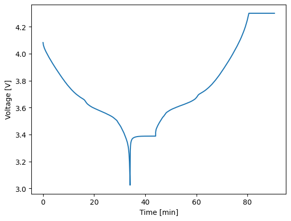
As an example, lets use an experiment that discharges at 2C until 3V, rests for 10 min, charges at 2C until 4.3V and then performs a voltage hold at 4.3V for 10 min. When using run_step we will run the steps in order and collect each step’s solution in a list, as shown below. After the loop we print the first solution to see what information is available.

sim = bm.SPM.Simulation()

expr = bm.Experiment()
expr.add_step('current_C', 2., (3600., 10.), limits=('voltage_V', 3.))
expr.add_step('current_C', 0., (600., 5.))
expr.add_step('current_C', -2., (3600., 10.), limits=('voltage_V', 4.3))
expr.add_step('voltage_V', 4.3, (600., 5.))

step_solns = []
for i in range(expr.num_steps):
    step_soln = sim.run_step(expr, i)
    step_solns.append(step_soln)
    
print(step_solns[0])

[bmlite UserWarning] SPM Simulation: Using default graphite_nmc532.yaml

StepSolution(
    solvetime=0.346 s,
    success=True,
    status=2,
    nfev=1396,
    njev=151,
    vars=['an', 'ca', 'el', 'time_s', 'time_min', 'time_h', 'current_A',
          'current_C', 'voltage_V', 'power_W'],
)

From the output above you can see that the first step was successful, how long it took to solve, and some additional details. Generally, running step-by-step can be valuable when you need to pause between steps to perform some analysis, inform later steps, or to help refine solver options for a given step.

There are a couple important thing to understands about how a Simulation runs experiments. When you first initialize a Simulation instance, the internal state is set to an equilibrium condition based on the initial intercalation fractions you defined in your .yaml file. When you run using run_step, the internal state of the Simulation is saved at the end of each step. This allows the next step to pick up from where the last step left off. If at any time you want to reset the state of your simulation back to the original initial equilibrium condition, you can use the pre method, which will re-run the preprocessing steps to re-initialize the instance. Since we will demonstrate the run method below using the same sim instance created above, we will use this approach to reset the simulation.

sim.pre()

Now let’s re-run the same experiment using the run method. The run method loops through all steps for you and returns a single solution that stitches together the step solutions rather than returning separate solutions for each step.

Note that the default behavior of run also automatically calls pre at the end of the last step. You can disable this using the optional reset_state=False argument. There are cases where you likely would and would not want the state to reset for you like this, which is why the option is exposed. For example, if you are validating a model and just sweeping through variable-rate discharge experiments, then there is no real need to every perform a charging simulation. In such a case, you should let reset_state=True so that the simulation always resets to a charged condition before running the next discharge experiment, which the need to waste time simulating the charge. On the other hand, if you want to define a complex series of experiments in which you want the state of the simulation to be passed from one to the next, then you would want to turn off this reset. As an example, maybe you want to define your discharge and charge steps separately in two Experiment instances rather than defining them all in one.

cycle_soln = sim.run(expr)

print(cycle_soln)

CycleSolution(
    solvetime=0.852 s,
    success=[True, True, True, True],
    status=[2, 1, 2, 1],
    nfev=[1396, 136, 1704, 80],
    njev=[151, 16, 206, 15],
    vars=['an', 'ca', 'el', 'time_s', 'time_min', 'time_h', 'current_A',
          'current_C', 'voltage_V', 'power_W'],
)

You can see the difference in the output above compared to the run_step solutions. When run is used, a CycleSolution instance is returned, which has list elements for “success” and its other metrics. Each index in these lists corresponds to a step in the experiment, so here we can see that all steps were successful. The status tells us that some steps terminated due to limits/events (status=2) while others stopped by reaching their final step time (status=1). You can see the human-readle status messages by also printing the message attribute. These are not included in the default printing to reduce clutter.

Regardless of which run method you choose, the solution instances can also be broken apart or stitched together. To stitch together the step solutions, pass them to the CycleSolution constructor from the model subpackage you are using. Breaking apart a cycle solution is achieved using its get_steps method, which can slice out a single step, or a portion of connected steps between two given indices. This provides a lot of flexibility in the interface, since you can also move between run and run_step as needed depending on how complicated your experiment and analysis are.

combined_soln = bm.SPM.CycleSolution(*step_solns)

print(combined_soln)

split_steps = [cycle_soln.get_steps(i) for i in range(expr.num_steps)]

print(split_steps[0])

CycleSolution(
    solvetime=0.853 s,
    success=[True, True, True, True],
    status=[2, 1, 2, 1],
    nfev=[1396, 136, 1704, 80],
    njev=[151, 16, 206, 15],
    vars=['an', 'ca', 'el', 'time_s', 'time_min', 'time_h', 'current_A',
          'current_C', 'voltage_V', 'power_W'],
)
StepSolution(
    solvetime=0.349 s,
    success=True,
    status=2,
    nfev=1396,
    njev=151,
    vars=['an', 'ca', 'el', 'time_s', 'time_min', 'time_h', 'current_A',
          'current_C', 'voltage_V', 'power_W'],
)

1.5. Final Thoughts

There are a variety of things you can learn from these models and their solutions. You will want to read through and understand more about the Solution classes if you want access to all of the internal state variables. The vars list in the example outputs above helps a bit with this. These are the keywords in the solution’s vars dictionary. This dictionary stores the sliced solution variables for each domain and some other helpful information like the time, current, and voltage values. However, the sliced state variables are not generated automatically. This is done to limit memory usage. To force the solution to post-process all of the variables, run the post method. Additional details on a domain’s state variables can be found in the bm.SPM.domains module.

If you are mostly only analyzing time, current, voltage, and/or power, then you likely won’t need to dig into the domains module. Instead, you might be more interested in using some built-in plotting functions to quickly visualize results. For this purpose, all Solution classes have a simple_plot method that takes plots any two of the non-domain vars keys against one another. For example, below we use the combined_soln from above to plot the full timeseries voltage data.

combined_soln.simple_plot('time_min', 'voltage_V')